Lensing in spherically symmetric and static spacetimes

4.3 Lensing in spherically symmetric and static spacetimes

The class of spherically symmetric and static spacetimes is of particular relevance in view of lensing, because it includes models for non-rotating stars and black holes (see Sections 5.1, 5.2, 5.3), but also for more exotic objects such as wormholes (see Section 5.4), monopoles (see Section 5.5), naked singularities (see Section 5.6), and Boson or Fermion stars (see Section 5.7). Here we collect the relevant formulas for an unspecified spherically symmetric and static metric. We find it convenient to write the metric in the form

As Equation (69

) is a special case of Equation (61

), all results of Section 4.2 for conformally stationary metrics apply. However, much stronger results are possible because for metrics of the form (69

) the geodesic equation is completely integrable. Hence, all relevant quantities can be determined explicitly in terms of integrals over the metric coefficients.

Redshift and Fermat geometry.
Comparison of Equation (69 ) with the general form (61 ) of a conformally stationary spacetime shows that here the redshift potential $f$ is a function of $r$ only, the Fermat one-form $ˆ ϕ$ vanishes, and the Fermat metric $ˆg$ is of the special form

By Fermat’s principle, the geodesics of $ˆg$ coincide with the projection to 3-space of light rays. The travel time (in terms of the time coordinate $t$ ) of a lightlike curve coincides with the $ˆg$ -arclength of its projection. By symmetry, every $ˆg$ -geodesic stays in a plane through the origin. From Equation (70

) we read that the sphere of radius $r$ has area $2 4πR (r)$ with respect to the Fermat metric. Also, Equation (70

) implies that the second fundamental form of this sphere is a multiple of its first fundamental form, with a factor $− R ′(r) (R(r)S (r ))− 1$ . If

the sphere $r = rp$ is totally geodesic, i.e., a $ˆg$ -geodesic that starts tangent to this sphere remains in it. The best known example for such a light sphere or photon sphere is the sphere $r = 3m$ in the Schwarzschild spacetime (see Section 5.1). Light spheres also occur in the spacetimes of wormholes (see Section 5.4). If $R ′′(r ) < 0 p$ , the circular light rays in a light sphere are stable with respect to radial perturbations, and if $′′ R (rp) > 0$ , they are unstable like in the Schwarschild case. The condition under which a spherically symmetric static spacetime admits a light sphere was first given by Atkinson [13

]. Abramowicz [1 ] has shown that for an observer traveling along a circular light orbit (with subluminal velocity) there is no centrifugal force and no gyroscopic precession. Claudel, Virbhadra, and Ellis [59

] investigated, with the help of Einstein’s field equation and energy conditions, the amount of matter surrounded by a light sphere. Among other things, they found an energy condition under which a spherically symmetric static black hole must be surrounded by a light sphere. A purely kinematical argument shows that any spherically symmetric and static spacetime that has a horizon at $r = rH$ and is asymptotically flat for $r → ∞$ must contain a light sphere at some radius between $rH$ and $∞$ (see Hasse and Perlick [152

]). In the same article, it is shown that in any spherically symmetric static spacetime with a light sphere there is gravitational lensing with infinitely many images. Bozza [37

] investigated a strong-field limit of lensing in spherically symmetric static spacetimes, as opposed to the well-known weak-field limit, which applies to light rays that come close to an unstable light sphere. (Actually, the term “strong-bending limit” would be more appropriate because the gravitational field, measured in terms of tidal forces, need not be particularly strong near an unstable light sphere.) This limit applies, in particular, to light rays that approach the sphere $r = 3m$ in the Schwarzschild spacetime (see [39

] and, for illustrations, Figures 15

, 16

, and 17

Index of refraction and embedding diagrams.
Transformation to an isotropic radius coordinate $&tidle;r$ via

takes the Fermat metric (70

) to the form

where

On the right-hand side $r$ has to be expressed by $&tidle;r$ with the help of Equation (72

). The results of Section 4.2 imply that the lightlike geodesics in a spherically symmetric static spacetime are equivalent to the light rays in a medium with index of refraction (74

) on Euclidean 3-space. For arbitrary metrics of the form (69

), this result is due to Atkinson [13

]. It reduces the lightlike geodesic problem in a spherically symmetric static spacetime to a standard problem in ordinary optics, as treated, e.g., in [213 ], §27, and [198 ], Section 4. One can combine this result with our earlier observation that the integral in Equation (67

) has the same form as the functional in Maupertuis’ principle in classical mechanics. This demonstrates that light rays in spherically symmetric and static spacetimes behave like particles in a spherically symmetric potential on Euclidean 3-space (cf., e.g., [104

]). If the embeddability condition

is satisfied, we define a function $Z (r)$ by

Then the Fermat metric (70

) reads

If restricted to the equatorial plane $𝜗 = π∕2$ , the metric (77

) describes a surface of revolution, embedded into Euclidean 3-space as

Such embeddings of the Fermat geometry have been visualized for several spacetimes of interest (see Figure 11

for the Schwarzschild case and [159

] for other examples). This is quite instructive because from a picture of a surface of revolution one can read the qualitative features of its geodesics without calculating them. Note that Equation (72

) defines the isotropic radius coordinate uniquely up to a multiplicative constant. Hence, the straight lines in this coordinate representation give us an unambiguously defined reference grid for every spherically symmetric and static spacetime. These straight lines have been called triangulation lines in [62 , 63 ], where their use for calculating bending angles, exactly or approximately, is outlined.

Light cone.
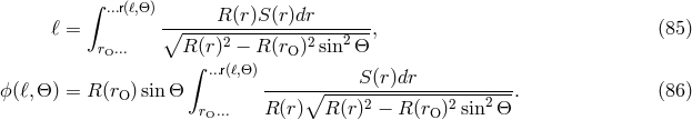
In a spherically symmetric static spacetime, the (past) light cone of an event $p O$ can be written in terms of integrals over the metric coefficients. We first restrict to the equatorial plane $𝜗 = π ∕2$ . The $ˆg$ -geodesics are then determined by the Lagrangian

For fixed radius value $rO$ , initial conditions

r(0) = r , dr(0) = cos-Θ-, O dℓ S (rO ) dφ sin Θ (80 ) φ(0) = 0, ---(0) = ------ d ℓ R (rO)

determine a unique solution $r = r(ℓ,Θ )$ , $φ = ϕ(ℓ,Θ)$ of the Euler–Lagrange equations. $Θ$ measures the initial direction with respect to the symmetry axis (see Figure 6

). We get all light rays issuing from the event $r = rO$ , $φ = 0$ , $𝜗 = π∕2$ , $t = tO$ into the past by letting $Θ$ range from 0 to $π$ and applying rotations around the symmetry axis. This gives us the past light cone of this event in the form

( ) tO − ℓ | r(ℓ,Θ )sin ϕ(ℓ,Θ )cos Ψ| (ℓ,Ψ,Θ ) ↦−→ |( |) . (81 ) r(ℓ,Θ )sinϕ(ℓ,Θ )sinΨ r(ℓ,Θ) cosϕ(ℓ,Θ )

$Ψ$ and $Θ$ are spherical coordinates on the observer’s sky. If we let $tO$ float over $ℝ$ , we get the observational coordinates (4

) for an observer on a $t$ -line, up to two modifications. First, $t O$ is not the same as proper time $τ$ ; however, they are related just by a constant,

Second, $ℓ$ is not the same as the affine parameter $s$ ; along a ray with initial direction $Θ$ , they are related by

The constants of motion

give us the functions $r(ℓ,Θ )$ , $ϕ(ℓ,Θ )$ in terms of integrals,

∫ ...r(ℓ,Θ) ℓ = ∘-----R-(r)S-(r)dr------, (85 ) rO... R (r)2 − R (rO)2sin2Θ ∫ ...r(ℓ,Θ) ϕ (ℓ,Θ) = R (r )sinΘ -----∘-----S(r)dr-----------. (86 ) O rO... R (r) R (r)2 − R (rO)2sin2Θ

Here the notation with the dots is a short-hand; it means that the integral is to be decomposed into sections where $r(ℓ,Θ )$ is a monotonous function of $ℓ$ , and that the absolute value of the integrals over all sections have to be added up. Turning points occur at radius values where $R (r) = R (rO) sin Θ$ and $R ′(r) ⁄= 0$ (see Figure 9

). If the metric coefficients $S$ and $R$ have been specified, these integrals can be calculated and give us the light cone (see Figure 12

for an example). Having parametrized the rays with $ˆg$ -arclength (= travel time), we immediately get the intersections of the light cone with hypersurfaces $t = constant$ (“instantaneous wave fronts”); see Figures 13

, 18

, and 19

Exact lens map.
Recall from Section 2.1 that the exact lens map [122 ] refers to a chosen observation event $pO$ and a chosen “source surface” $𝒯$ . In general, for $𝒯$ we may choose any 3-dimensional submanifold that is ruled by timelike curves. The latter are to be interpreted as wordlines of light sources. In a spherically symmetric and static spacetime, we may take advantage of the symmetry by choosing for $𝒯$ a sphere $r = rS$ with its ruling by the $t$ -lines. This restricts the consideration to lensing for static light sources. Note that all static light sources at radius $rS$ undergo the same redshift, $log(1 + z) = f(rS) − f(rO)$ . Without loss of generality, we place the observation event $pO$ on the 3-axis at radius $r O$ . This gives us the past light cone in the representation (81 ). To each ray from the observer, with initial direction characterized by $Θ$ , we can assign the total angle $Φ(Θ )$ the ray sweeps out on its way from $rO$ to $rS$ (see Figure 6 ). $Φ(Θ )$ is given by Equation (86 ),

where the same short-hand notation is used as in Equation (86

). $Φ (Θ )$ is not necessarily defined for all $Θ$ because not all light rays that start at $rO$ may reach $rS$ . Also, $Φ(Θ )$ may be multi-valued because a light ray may intersect the sphere $r = rS$ several times. Equation (81

) gives us the (possibly multi-valued) lens map

( r sin Φ(Θ )cos Ψ) ( S ) (Ψ,Θ ) ↦−→ rS sin Φ(Θ )sinΨ . (88 ) rScos Φ(Θ )

It assigns to each point on the observer’s sky the position of the light source which is seen at that point. $Φ (Θ)$ may take all values between 0 and infinity. For each image we can define the order

which counts how often the ray has met the axis. The standard example where images of arbitrarily high order occur is the Schwarzschild spacetime (see Section 5.1). For many, though not all, applications one may restrict to the case that the spacetime is asymptotically flat and that $rO$ and $rS$ are so large that the spacetime is almost flat at these radius values. For a light ray with turning point at $rm (Θ)$ , Equation (87

) can then be approximated by

If the entire ray remains in the region where the spacetime is almost flat, Equation (90

) gives the usual weak-field approximation of light bending with $Φ(Θ )$ close to $π$ . However, Equation (90

) does not require that the ray stays in the region that is almost flat. The integral in Equation (90

) becomes arbitrarily large if $rm (Θ )$ comes close to an unstable light sphere, $R ′(rp) = 0$ and $R ′′(rp) > 0$ . This situation is well known to occur in the Schwarzschild spacetime with $rp = 3m$ (see Section 5.1, in particular Figures 9

, 14

, and 15

). The divergence of $Φ (Θ)$ is always logarithmic [37

]. Virbhadra and Ellis [336

] (cf. [338

] for an earlier version) approximately evaluate Equation (90

) for the case that source and observer are almost aligned, i.e., that $Φ(Θ )$ is close to an odd multiple of $π$ . This corresponds to replacing the sphere at $rS$ with its tangent plane. The resulting “almost exact lens map” takes an intermediary position between the exact treatment and the quasi-Newtonian approximation. It was originally introduced for the Schwarzschild metric [336

] where it approximates the exact treatment remarkably well within a wide range of validity [118

]. On the other hand, neither analytical nor numerical evaluation of the “almost exact lens map” is significantly easier than that of the exact lens map. For situations where the assumption of almost perfect alignment cannot be maintained the Virbhadra–Ellis lens equation must be modified (see [70

]; related material can also be found in [38

]).

Figure 6: Illustration of the exact lens map in spherically symmetric static spacetimes. The picture shows a spatial plane. The observation event (dot) is at $r = rO$ , static light sources are distributed at $r = r S$ . $Θ$ is the colatitude coordinate on the observer’s sky. It takes values between 0 and $π$ . $Φ (Θ )$ is the angle swept out by the ray with initial direction $Θ$ on its way from $rO$ to $rS$ . It takes values between 0 and $∞$ . In general, neither existence nor uniqueness of $Φ (Θ)$ is guaranteed for given $Θ$ . A similar picture is in [271

4.3.0.1 Distance measures, image distortion and brightness of images.

For calculating image distortion (see Section 2.5) and the brightness of images (see Section 2.6) we have to consider infinitesimally thin bundles with vertex at the observer. In a spherically symmetric and static spacetime, we can apply the orthonormal derivative operators $∂Θ$ and $sin Θ ∂Ψ$ to the representation (81

) of the past light cone. Along each ray, this gives us two Jacobi fields $Y1$ and $Y2$ which span an infinitesimally thin bundle with vertex at the observer. $Y1$ points in the radial direction and $Y 2$ points in the tangential direction (see Figure 7

). The radial and the tangential direction are orthogonal to each other and, by symmetry, parallel-transported along each ray. Thus, in contrast to the general situation of Figure 3

, $Y1$ and $Y2$ are related to a Sachs basis $(E1, E2)$ simply by $Y1 = D+E1$ and $Y2 = D − E2$ . The coefficients $D+$ and $D −$ are the extremal angular diameter distances of Section 2.4 with respect to a static observer (because the $(Ψ, Θ )$ -grid refers to a static observer). In the case at hand, they are called the radial and tangential angular diameter distances. They can be calculated by normalizing $Y1$ and $Y2$ ,

∘ -------------------------- f(r(ℓ,Θ)) 2 2 2 D+ (ℓ,Θ ) = e R(rO )cosΘ R (r(ℓ,Θ)) − R (rO)sin Θ ∫ ...r(Θ,ℓ) S (r)R(r)dr × ∘----------------------3, (91 ) rO... R (r)2 − R (rO)2sin2Θ sinϕ (ℓ,Θ ) D − (ℓ,Θ ) = ef(r(ℓ,Θ))R (r(ℓ,Θ ))----------. (92 ) sin Θ

These formulas have been derived first for the special case of the Schwarzschild metric by Dwivedi and Kantowski [84

] and then for arbitrary spherically symmetric static spacetimes by Dyer [85

]. (In [85

], Equation (92

) is erroneously given only for the case that, in our notation, 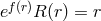$f(r) e R(r) = r$ .) From these formulas we immediately get the area distance $∘ -------- Darea = |D+D − |$ for a static observer and, with the help of the redshift $z$ , the luminosity distance $Dlum = (1 + z )2Darea$ (recall Section 2.4). In this way, Equation (91

) and Equation (92

) allow to calculate the brightness of images according to the formulas of Section 2.6. Similarly, Equation (91

) and Equation (92

) allow to calculate image distortion in terms of the ellipticity $𝜀$ (recall Section 2.5). In general, $𝜀$ is a complex quantity, defined by Equation (49

). In the case at hand, it reduces to the real quantity $𝜀 = D − ∕D+ − D+ ∕D −$ . The expansion $𝜃$ and the shear $σ$ of the bundles under consideration can be calculated from Kantowski’s formula [172 , 84

to which Equation (27

) reduces in the case at hand. The dot (= derivative with respect to the affine parameter $s$ ) is related to the derivative with respect to $ℓ$ by Equation (83

). Evaluating Equations (91

, 92

) in connection with the exact lens map leads to quite convenient formulas, for static light sources at $r = rS$ . Setting $r(ℓ,Θ ) = rS$ and $ϕ(ℓ,Θ ) = Φ(Θ )$ and comparing with Equation (87

) yields (cf. [271

])

These formulas immediately give image distortion and the brightness of images if the map $Θ ↦→ Φ (Θ )$ is known.

Figure 7: Thin bundle around a ray in a spherically symmetric static spacetime. The picture is purely spatial, i.e., the time coordinate $t$ is not shown. The ray is contained in a plane, so there are two distinguished spatial directions orthogonal to the ray: the “radial” direction (in the plane) and the “tangential” direction (orthogonal to the plane). For a bundle with vertex at the observer, the radial diameter of the cross-section gives the radial angular diameter distance $D+$ , and the tangential diameter of the cross-section gives the tangential angular diameter distance $D−$ . In contrast to the general situation of Figure 3

, here the angle $χ$ is zero (if the Sachs basis $(E ,E ) 1 2$ is chosen appropriately). Recall that $D+$ and $D −$ are positive up to the first caustic point.

Caustics of light cones.
Quite generally, the past light cone has a caustic point exactly where at least one of the extremal angular diameter distances $D+$ , $D −$ vanishes (see Sections 2.2, 2.3, and 2.4). In the case at hand, zeros of $D+$ are called radial caustic points and zeros of $D −$ are called tangential caustic points (see Figure 8 ). By Equation (92 ), tangential caustic points occur if $ϕ(ℓ,Θ )$ is a multiple of $π$ , i.e., whenever a light ray crosses the axis of symmetry through the observer (see Figure 8 ). Symmetry implies that a point source is seen as a ring (“Einstein ring”) if its worldline crosses a tangential caustic point. By contrast, a point source whose wordline crosses a radial caustic point is seen infinitesimally extended in the radial direction. The set of all tangential caustic points of the past light cone is called the tangential caustic for short. In general, it has several connected components (“first, second, etc. tangential caustic”). Each connected component is a spacelike curve in spacetime which projects to (part of) the axis of symmetry through the observer. The radial caustic is a lightlike surface in spacetime unless at points where it meets the axis; its projection to space is rotationally symmetric around the axis. The best known example for a tangential caustic, with infinitely many connected components, occurs in the Schwarzschild spacetime (see Figure 12 ). It is also instructive to visualize radial and tangential caustics in terms of instantaneous wave fronts, i.e., intersections of the light cone with hypersurfaces $t = constant$ . Examples are shown in Figures 13 , 18 , and 19 . By symmetry, a tangential caustic point of an instantaneous wave front can be neither a cusp nor a swallow-tail. Hence, the general result of Section 2.2 implies that the tangential caustic is always unstable. The radial caustic in Figure 19 consists of cusps and is, thus, stable.

Figure 8: Tangential and radial caustic points. Tangential caustic points, $D − = 0$ , occur on the axis of symmetry through the observer. A (point) source at a tangential caustic point is seen as a (1-dimensional) Einstein ring on the observer’s sky. A point source at a radial caustic point, $D+ = 0$ , appears “infinitesimally extended” in the radial direction.